DyingLoveGrape.

Applying Topology to Data, Part 1: A Brief Introduction to Abstract Simplicial and Čech Complexes.

Prereqs.

The construction of the complex won't use all that much topology but the main application I will be working towards is topological in nature. For this first post I'm going to be defining most of the concepts I work with, but once we begin some of the more advanced material (in the upcoming posts) I'll begin to assume more — though, I'll try to link to relevant resources as best I can!

Tiny Introduction.

Lately, I've been considering some different kinds of structures which can be put on data — in particular, Delaunay Diagrams provide such a structure given some set of points in a dataset (or otherwise). Gunnar Carlsson's paper Topology and Data (available here) is an excellent introduction for working with data using topology; we will follow Dr. Carlsson's lead and begin by talking about Čech complexes. They're pretty neat in their own right, too. In This post, we'll talk about some of the topics we need to introduce Čech complexes: simplicial and abstract simplicial complexes, open and "good" open covers, and the nerve of a cover.

Simplicial and Abstract Simplicial Complexes.

The idea behind a Simplicial Complex is that you take a ton of points, edges, triangles, and hyper-dimensional triangles and glue them together nicely along the edges to make nice things. For example, one can think of a disco ball (made with triangles of glass instead of squares) as a simplicial complex which approximates a sphere. Here's another one which is called the (hollow) octohedron:

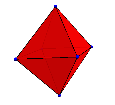
Anyone who has played early 3D video games, such as Playstation 1 or N64 games, will remember the blocky and polygonal structures which made up the characters; in general, 3D models are made by making a simplicial shell (which approximates a "real shape" like a sphere, a face, etc.) and then filling them in. Note, though, that we cannot simply draw every possible angle that the simplicial shell will be looked at: we usually plug in coordinates and where we are looking from and tell the program (Maya, Mathematica, ete.) to calculate how the structure should be shown to us. For example, I made the above figure by telling Mathematica to draw triangles at certain vertices and fill them in with nice red coloring; I could even rotate them in Mathematica, which looked quite nice!

[If I figure out a way to embed it nicely in this page, I'll let you rotate it too! Otherwise, just check out a page like this; note, you must allow javascript to run by clicking on the figures or by having it enabled in your browser!]

Let's consider the following question: If I have tons of points, edges, and triangles, how do I keep track of what things are adjacent to each other? One particularly nice way is the following:

• Number the vertices $1,2,3,\dots, n$.
• For each edge you want, make a set of the vertices it is between. For example, $\{1,2\}$ is an edge between vertex 1 and vertex 2.
• For each triangle you want, make a set of the vertices it includes. For example, $\{1,2,3\}$ is a triangle using vertex 1, vertex 2, and vertex 3.
• Make a set, which we'll call $\Sigma$, which is the union of all of the points, edges, and triangles you have. That is, \[\Sigma = \mbox{Vertex Set}\cup \mbox{Edge Set}\cup \mbox{Triangle Set}.\]

For example,

We note that here we have the following points: \[\{1,2,3,4,5\}.\] We note also that we have the following edges: \[\{\{1,2\},\{1,3\}, \{2,3\}, \{3,4\}, \{2,4\}, \{4,5\}\}.\] Last, we note that we only want the following triangle: \[\{1,2,3\},\] even though it "looks" like we have a triangle $\{2,3,4\}$, we have noted (by not coloring it in) that it is not part of our simplicial complex. Therefore, we have a bunch of points, a few lines, and a single face. If we'd colored in $\{2,3,4\}$ like $\{1,2,3\}$, then it, too, would be one of our faces. Alas, it is not. The way we talk about this particular simplicial complex in an abstract sense is: \[\begin{align*}\Sigma = &\{1,2,3,4,5,\{1,2\},\{1,3\}, \{2,3\}, \{3,4\},\\ &\{2,4\}, \{4,5\}, \{1,2,3\}\}.\end{align*}\]

[Note: Strictly speaking, we should probably be writing $\{1\}, \{2\},\dots$ for the vertices, since these must also be subsets, but we are abusing notation here slightly and simply writing $1,2,3,\dots$. Just keep this in mind, but it shouldn't mess too much up.]

Note that this completely characterizes our simplex if we don't really care how long the edges are, how the points are arranged, etc. so long as everything is connected right and all the pieces (perhaps resized or rotated a bit!) are there. For example, we could also make the following picture from the data given in our abstract simplicial complex above:

Notice that, up to some squishing the edges and rotating stuff around and resizing some things, this is the same simplex as what we started with in terms of the right edges being connected to the right vertices and the right triangles filled in.

But, we'd also like to be able to go in the opposite direction: we'd like to build an abstract simplicial complex and have it represent some real complex. But not every abstract simplicial complex works. For example, \[\{1,2,3,\{1,2,3\}\}\] is not an abstract simplicial complex; why not? The reason is because there are no edges for the triangle $\{1,2,3\}$ to be bounded by! We'd need $\{1,2\}, \{1,3\}$ and $\{2,3\}$ to be in the set in order for this to be defined. In the case of simplicial complexes, we need all of the edges to be accounted for if we're going to include something which needs those edges. Another non-example would be something like \[\{1,2,\{1,2\}, \{1,3\}, \{2,3\}, \{1,2,3\}\}\] Here, we're making a reference to some vertex called "$3$" which isn't actually in the simplex; we can't allow that! Hence,

If a set $A$ is in our abstract simplicial complex, so is each of its non-empty subsets.

This is exactly what we noted above. If we have a triangle, we need all of its edges and vertices to be in the abstract simplicial complex. In fact, this is the only major restriction we need to put on ourselves to be able to start constructing our abstract simplicial complexes. Let's formally define this now

Definition (Abstract Simplicial Complex). Let $V = \{1,2,\dots, n\}$. Let $\Sigma$ be a set of non-empty subsets of $V$. We call $\Sigma$ an Abstract Simplicial Complex if it has the following property: whenever a set $A\in \Sigma$, every nonempty subset of $A$ is also an element of $\Sigma$.

Notice that there's nothing here that says we've got to stay in two dimensions: we've, so far, used points, lines, and triangles, but there is nothing keeping us from using higher-dimensional objects. Indeed, if we wanted to, we could extend the notion of "triangle" into higher dimensions (the third dimensional one, for example, being the tetrahedron) and we will eventually do this. For most of what we will do, it will suffice to work with points, lines, and triangles, but note that there is no real difficulty in extending our abstract simplicial complexes beyond this.

As usual, there's the concept of a subcomplex of an abstract simplicial complex and, as usual, it's simply a structure $\Gamma\subseteq \Sigma$ which is, itself, an abstract simplicial complex.

Slightly more interesting is the notion of an $n$-skeleton. We'll illustrate this first with an example. Take the simplicial complex below:

As before, we can construct the abstract simplicial complex which represents this simplicial complex; the reader ought to do this for practice. Here's the answer when you're done:

\[\begin{align*} \Sigma =&\{1,2,3,4,5,6,7,\{1,2\},\{2,3\},\\ &\{2,7\},\{3,4\},\{3,7\}, \{4,5\}, \{4,7\},\\ &\{5,7\}, \{6,7\}, \{2,3,7\}, \{4,5,7\}\}.\end{align*}\]

An $n$-skeleton of this structure is the collection which contains all of the objects in our simplicial structure which are at most $n$-dimensional: for example, the 0-skeleton is the set of vertices, the 1-skeleton is the set of edges and vertices, the 2-skeleton is the set of triangles, edges, and vertices. Let's look at a picture of these things. First, the 0-skeleton:

Just the vertices. Now the 1-skeleton:

We've added in the edges. Now the 2-skeleton:

This was, in our case, the original structure since we do not have any objects which are of dimension higher than 2 in our structure. Notice that each of these are subcomplexes. In fact, they are special subcomplexes: the $n$-skeleton creates a "frame" using only at most $n$ dimensional objects. This becomes useful when our structure is extremely large or extends into higher dimensions: it's almost like looking at the foundation of a house to see approximately what the house will look like.

Look at the $1$-skeleton again — haven't we seen things that look like this before? Of course! Graphs! Indeed, the $1$-skeleton of a simplicial complex is always a graph and, because of this, it is called the underlying graph of our subcomplex.

To generalize a bit...

We've already made Abstract Simplicial Complexes relatively general, but the language I've used wasn't as general. I just want to note the following, since it is language that will be used often in the subject.

Above, we talked about vertices, edges, triangles, and so forth, but we can define all of these as different dimensional cases of a particular concept: a simplex. There are a number of of rigorous definitions of what a simplex is, but I'll simply attempt to appeal to intuition:

• A $0$-simplex is a point.
• A $1$-simplex is a line segment (with two endpoints). It's, therefore, a line segment with two $0$-simplices at its endpoints.
• A $2$-simplex is a triangle. One can imagine putting two $1$-simplices on ${\mathbb R}^{2}$, the plane, both starting at the origin but one going to $(0,1)$ and the other going to $(1,0)$. We connect the vertices and then "fill in" the enclosed piece, making a triangle.
  
  
  
  
  
  
• A $3$-simplex is a solid tetrahedron. One can imagine three $1$-simplices on ${\mathbb R}^{3}$ all starting at the origin but going to $(0,0,1), (0,1,0),(1,0,0)$ respectively. One then connects all of the $0$-simplexes together with $1$-simplexes, as in the figure below:
  
  
  
  
  
  Next, solid triangles (2-simplexes) are placed in the four spots where the $1$-simplexes have made triangles: \[\begin{align*}\{(0,0,0), (0,0,1), (0,1,0)\},\\\{(0,0,0), (0,0,1), (1,0,0)\},\\ \{(0,0,0), (0,1,0), (1,0,0)\},\\\{(0,0,1), (0,1,0), (1,0,0)\}.\end{align*}\] Once this is done, one has a hollow tetrahedron. We now "fill in the middle" to make it a solid tetrahedron.
• In general, an $n$ simplex will have $n$ edges starting at the origin in ${\mathbb R}^{n}$ and going to $(0,0,\dots, 0,1,0,\dots, 0)$ with 0's everywhere and $1$ in the $i$-th place, for each edge (as we've done above). One then fills in some $2$-simplices, $3$-simplices, etc., up to $(n-1)$-simplices. Don't worry if you can't picture this — these structures are impossible for us to imagine without using clever tricks and, even these only allow us to imagine an approximation.

Another way to imagine an $n$ simplex is the following: consider ${\mathbb R}^{n+1}$ and place a point at $(1,0,0,\dots, 0), (0,1,0,\dots, 0)$, $\dots$, $(0,0, \dots, 0,1)$ and at the origin. Then take the convex hull (that is, create the smallest convex shape containing these points). The reader may want to do this for $1$-, $2$- and $3$-simplices to show that this gives the same structure. Neat.

A little bit of Simplex Practice...

Let's practice simplices by converting a simplicial complex into an abstract simplicial complex and, conversely, converting an abstract simplicial complex into a simplicial complex.

Given the following structure, we need to identify all of the simplices which are used. To make it easier, I've included the 1-skeleton below it — remember that this is just the collection of $0$- and $1$-simplices in our simplicial complex.

Note that in the simplicial complex, I've drawn the figure on the left-hand side in darker blue to denote that it is a "solid tetrahedron" (that is, a 3-simplex). Let's begin with the $0$-simplices, since they're often the easiest to write down. In this case, we have \[\{1,2,3,4,5,6,7,8,9\}\] as our set of $0$-simplices. Looking at the $1$-skeleton gives us an idea of the $1$-simplices we have. They are \[\begin{align*}&\{\{1,2\}, \{1,3\}, \{1,4\}, \{2,4\},\\ &\{3,5\},\{5,6\},\{6,7\},\{5,7\},\\ &\{5,8\}, \{8,7\}, \{7,9\}\}\end{align*}\] At last, looking at the simplicial complex will allow us to see what $2$-simplices we have. Remember that there are a few bounding the solid tetrahedron on the left-hand side! Hence, we have the $2$-simplices are \[\{\{1,2,3\}, \{1,2,4\}, \{1,3,4\}, \{2,3,4\}, \{5,6,7\}\}\] and that's all. Last, the solid tetrahedron on the left-hand side is our only $3$-simplex. Such a lonely solid tetrahedron. Either way, our $3$-simplices are therefore just \[\{\{1,2,3,4\}\}.\] To make the abstract simplicial complex from this, we simply union all of these things together. Hence, the whole thing is: \[\begin{align*} \Sigma = &\{1,2,3,4,5,6,7,8,9,\\ &\{1,2\}, \{1,3\}, \{1,4\}, \{2,4\},\\ &\{3,5\},\{5,6\},\{6,7\},\{5,7\},\\ &\{5,8\}, \{8,7\}, \{7,9\}\\ &\{1,2,3\}, \{1,2,4\}, \{1,3,4\},\\ &\{2,3,4\}, \{5,6,7\}, \{1,2,3,4\}\} \end{align*}\] Neat. Now, let's do the reverse and make a structure out of some abstract simplicial complex. Let's let our new complex (which we'll call $\Sigma_{2}$ so as not to confuse it with the previous complex) be defined by \[\begin{align*} \Sigma_{2} = &\{1,2,3,4,5,\\ &\{1,2\}, \{1,3\}, \{1,4\}, \{2,4\},\\ &\{2,5\}, \{1,2,3\}, \{1,2,4\}, \{1,3,4\},\\ &\{2,3,4\}, \{1,2,3,4\}\} \end{align*}\] We first draw out the $0$- and $1$ simplices, since they're the easiest to draw out first (note that this makes the $1$-skeleton of our simplicial complex),

Now, let's put on our $2$-simplices. This'll make our $2$-skeleton.

Note that we've put four of them up, making a hollow tetrahedron on the top. The last thing we need to do is add our $3$-simplex, which will "fill in" the tetrahedron and make it into a solid tetrahedron, which I've attempted to draw using the darker blue color here:

Note that this simplicial complex is not the unique one that can be made form our abstract simplicial complex: we could have made some edges longer, put some vertices in other places, and even bent some lines, warped some triangles, etc., but so long as all of the pieces are connected to the correct pieces this is a good representation of our abstract simplicial complex.

Open Coverings and Contractible Spaces.

If you aren't familiar with basic topology, you may want to familiarize yourself with the gist of it [notes by Allen Hatcher]. Otherwise, you may recall the notion of an open cover:

Definition (Open Cover). Given a topological space $X$, an open cover of $X$ is a set $\{U_{i}\}_{i}$ of open sets with the property that for each $x\in X$ there is some $U_{j}$ in our set such that $x\in U_{j}$.

If you think of the space $X$ as someone's body and the open sets as patches of fabric, then the open cover would literally be covering the entire person's body with the patches of fabric. The open cover "covers" the space, and each of the pieces is open.

There's a number of different, equally nice covers for any particular set $X$. For example, to cover the interval $[0,1]\subseteq{\mathbb R}$ we could use the collection of open sets \[\{(-1,\tfrac{1}{2}), (0,\tfrac{3}{4}), (\tfrac{1}{2},2)\}\] or we could use the collection \[\{(-\infty, \tfrac{1}{2}), (0,\infty)\}\] or even just the single open set \[\{(-3,3)\}.\] Each of these covers is fine, but for our purposes we'd like to restrict the kinds of covers we'll allow. Because of this, we'd like to define a particularly nice kind of space called a contractible space. The gist of a contractible space is this: it's one where you can squish it down to a point without filling in any holes or squishing two different disjoint components of the space together. We'll make this mathematically precise in a moment, but let's just look at a few spaces on the plane ${\mathbb R}^{2}$ to make this point a bit more clear.

The following two spaces are each constractible. Notice that there's only one component to each, and that there aren't any "holes" inside them. If you didn't have to conserve the area, you could easily squish them down to a single point.

On the other hand, these three spaces are not contractible. The first has a hole in the middle, which we cannot fill (we could, though, squish this down into a circle!). The second has two different components; we could contract each component down to a point, but we can't squish the two points down to a single point — the best we can do with this space is to compress it down to two distinct points. The last picture has both problems: more than one piece, and some holes in them.

This is the general idea (at least in ${\mathbb R}^2$), but we ought to define this formally. The definition is going to be a bit strange, so let's talk for a moment about where it's coming from. If you don't care so much for the motivation, feel free to skip the next section which will delve a bit into the topology motivating the definition of contractible.

Brief Sidenote: Homotopies.

We're used to spaces having continuous maps between them; indeed, point-set topology courses teaches that, besides the "usual" continuous funcitons $f:{\mathbb R}\to{\mathbb R}$ we know from calculus, there are ways to extend the notion of continuity so that we can talk about $f:X\to Y$ being continuous even if we don't have a notion of a limit. A less common notion is that we can have continuous transformations between mappings; that is, we can take one continuous function and make it into another continuous function in a continuous manner. To help visualize this (before we formalize it) think about $f:(0,1)\to (0,1)$ defined by $f(x) = x^{2}$. If we, say, alter $f$ a bit and define $f_{1}(x) = 0.9x^{2}$, then this is looks fairly similar to $f(x)$; we may similarly define $f_{2}(x) = 0.8x^{2}, f_{3}(x) = 0.7x^{2}$ and so forth, until we get to $f_{10}(x) = 0$. Let's look at the images of these functions:

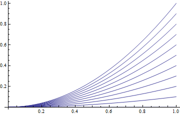
Notice that this "nicely" transforms $f(x) = x^{2}$ into the function $g(x) = 0$. If we were to let $f_{1}(x) = 0.99x^{2}$, $f_{2}(x) = 0.98x^{2}$ and so on, then our picture would look like this:

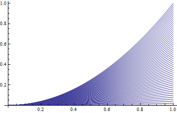
which looks "smoother". If we wanted, we could think of doing this transformation in real time: $f(x)$ is the function at $t = 0$, then at $t = 0.01$ we have $f_{1}(x)$, at $t = 0.02$ we have $f_{2}(x)$, and so forth, until we get to $g(x) = 0$ at $t = 1$; notice that the times I've picked are arbitrary and only were chosen to make the value of $t$ lie between 0 and 1; that is, $t\in [0,1]$. If we were to make the time intervals infinitely small, we'd have a continuous transformation between the functions $f(x) = x^{2}$ and $g(x) = 0$, so let's do just this. Instead of labeling infinitely many $f_{i}$'s, let's parameterize this by a new function $h(x,t)$ which we'll call a homotopy between $X$ and $Y$. Let's say that at $t = 0$ we want $h(x,0) = f(x)$, our original function, and at $t = 1$ we want $h(x,1) = g(x)$, the function we're transforming $f$ into. Inbetween these times, we want this function to be continuous. If such a function exists, then we say that $f$ and $g$ are homotopic mappings. Formally,

Definition (Homotopic Mappings). Continuous maps $f:X\to Y$ and $g:X\to Y$ are called homotopic if there exists a continuous function $h(x,t):X\times [0,1]\to Y$ such that $h(x,0) = f(x)$ and $h(x,1) = g(x)$. We denote this by $f\simeq g$. The function $h(x,t)$ is called a homotopy between $f$ and $g$.

We'll discuss this in more detail in the next post, but for now let's think about what the homotopy from our $f(x) = x^{2}$ to $g(x) = 0$ would be. At $t=0$ we'd like $h(x,0) = f(x) = x^{2}$, so let's try the function $h(x,t) = (1-t)x^{2}$. By coincidence, this also happens to satisfy $h(x,1) = (1-1)f(x) = 0$. Moreover, this function is continuous in both $x$ and $t$ (in the normal calculus sense) which is the last thing we needed to check. Hence, $f(x) = x^{2}$ and $g(x) = 0$ are homotopic. It may be the case, in the future, that our homotopies are not this easy to construct; nonetheless, many times we will be able to employ the "$(1-t)f(x) + tg(x)$" trick, which gives us $f(x)$ when $t = 0$ and $g(x)$ when $t = 1$.

At this point, we can talk about contractible spaces We need two little terms, and then we define it. A function $g:X\to Y$ is called a constant function if $g(x) = y_{0}$ for some point $y_{0}\in Y$. If a continuous function $f$ is homotopic to a constant function $g$ we call $f$ nullhomotopic. Given a space $X$, there exists an identify function from $X$ to itself which is denoted $1_{X}$ and is defined by $1_{X}(x) = x$; if $1_{X}$ is nullhomotopic, then we say that $X$ is contractible.

Whew. What does this mean? Well, it doesn't quite mean that we're squishing $X$ down. We're saying that the identity map of $X$ is continuously transformable to a constant mapping; hence, any continuous mapping which has $X$ as its domain or range will also be a constant mapping; why? If $k:X\to Y$ is a function, what is $k\circ 1_{X}$? Can you constuct a new homotopy using $h(x,t)$ which is $k$ at $t = 0$ and a constant at $t =1$? In a nutshell this means that, as far as any functions from or to $X$ are concerned, $X$ is just a point. Because we're "contracting" down $X$ in this way, we call $X$ contractible.

...So, why, in the above section, did I talk about holes and disconnected components if we aren't "really" shrinking down $X$? Visually, these things are obvious indicators that a space is not contractible; one can derive the fact that they are not contractible from the definition we give in this section. At times, it is easier to look at the features of a space to see if it has any obvious problems which would prevent it from being contractible.

Back to Open Covers and Contractible Spaces...

From the above, we finally are able to define a contractible space:

Definition (Nullhomotopic). A topological space $X$ is contractible if its identity mapping, $1_{X}:X\to X$ given by $1_{X}(x) = x$, is nullhomotopic.

Great. Good. You might be wondering at this point what any of this has to do with open coverings (remember, they're part of this section too!). Generally, the answer is: not much. But, because we want our open covers to be extra nice we must utilize the idea of contractibility. Let me define what, for us, will be called a good covering,

Definition (Good Open Covering). An open covering $\{U_{i}\}_{i}$ of a space $X$ is called a good open covering, or simply a good covering, of $X$ if all nonempty finite intersections $U_{i_{1}}\cap U_{i_{2}}\cap \cdots U_{i_{m}}$ are also contractible (including the sets $U_{i}$ themselves).

For now, let's work exclusively in ${\mathbb R}^{2}$, just because it's easier to visualize. Let's give some examples of good open covers and examples of "not so good" open covers; this'll give us some insight into why not all covers are good covers.

The space we'll cover is the circle, also called $S^{1}$ (or the 1-sphere). Note that an open set on $S^{1}$ would look like a "curved" open interval on the real line like this:

But because this is slightly hard to draw, we'll draw an open set in the plane ${\mathbb R}^{2}$, and one would get the open set on $S^{1}$ by intersecting this open set (blue colored below) with the space $S^{1}$. For example, the following picture would give the same open set on $S^{1}$ as the above picture.

Now that we know what our open sets will look like, let's draw a cover. What about just taking two big open sets and covering the top and the bottom of the circle?

This is certainly a cover, but is it a good cover? You should show that each of the open sets individually on the circle make a "curved open interval" and are, therefore, contractible. But, the intersection of the two open sets gives us:

Which, if you recall, intersected with $S^{1}$ looks sort of like:

There are two disjoint pieces of the intersection; as above, we noted that two disjoint pieces would not be contractible. Hence, this is not a good cover. On the other hand, look at the following cover:

Looks similar, but there are many more open sets on the circle. Each is contractible individually (as above), but let's look at the nonempty intersections. Each looks like this:

Which (on the circle) would look like a single little curved open interval. This is contractible. Because any three distinct open sets have empty intersection, this accounts for all the nonempty finite intersections. Hence, all finite nonempty intersections of the open sets are contractible. This means that this cover is a good cover. Neat.

Why is this cover any different from the other? The cover with more open sets perhaps gives us more local detail than the one with only two open sets; for a circle, this may not be obvious, but for a set with a number of intricate parts it may be the case that two open sets are too "coarse" to gather all of the neat little local detail. It would be sort of like the following situation: pretend you need to take a photo of the shoreline of a local beach, but you can only take one photo. You'd have to get in a helicopter and photograph the entire thing to get it in one photo. On the other hand, if you had one hundred photos you could get a great deal closer to the shoreline and could piece the photos together to make one very long photo with significantly more detail than the one photo had. Similarly, if you had a hundred thousand photos, you'd be able to get quite a large amount of detail from the shore if you took close-up photos and stitched the photos together.

This is an argument for "more open sets", but why the intersections-need-to-be-contractible criteria? This has to do with how our Čech Complexes will be constructed, since this will more accurately capture the "shape" of the space that the cover is covering. More specifically, we would like to be able to have an open cover of something and be able to somehow reconstruct something which is "similar to" the thing we're covering but is computationally easier to work with. In fact, at this point, it's quite easy to define exactly how to make this structure; let's not waste any more time and get right into it!

Nerves and Čech Complexes.

Given any cover (not necessarily a good cover), we can construct a nerve of the covering as follows:

[Note: The nerve can be made into a simplicial complex in the obvious way: using the relationships between the simplices to "build up" a real simplicial complex. We will be identifying the nerve with the simplicial complex created from its abstract simplicial complex.]

The idea, then, is to take a non-empty intersection of $k$ things and associate with that a $k$-simplex. Nerves, in general, are a useful tool in topology but, for us, we will want to use a specific kind of nerve. Specifically,

Definition (Čech Complex). Let $X$ be a topological space and $\{U_{i}\}_{i}$ be an open cover. If $\{U_{i}\}_{i}$ is a good cover (in the sense that we defined above) then we call its nerve ${\mathcal N}(\{U_{i}\}_{i})$ the Čech Complex of the covering $\{U_{i}\}_{i}$.

Let's just do a few examples before we end this first part.

Čech Complexes: Examples.

If we look at our good cover of $S^{1}$ above, we can construct the associated Čech Complex as follows:

Notice that the Čech Complex part is just the red parts: the five vertices and the edges between them. In this simple case, the simplicial complex it makes looks quite similar to a circle, as we would expect.

Let's try a more complicated space.

Note that I've already covered this space with a bunch of open sets; I also claim that this is a good cover. Let's see what information the Čech Complex will preserve about the space given this cover. First, let's draw the vertices:

Now we'll draw an edge between any two vertices where there's a nonempty intersection between their corresponding open sets, and we'll draw a triangle whenever there's a triple overlap. We obtain:

Which gives us the Čech Complex associated to the cover of this space. Without the background and such, it looks like this:

This begs the question: what was preserved about the underlying space? what wasn't preserved? We note that the shape and the size (as well as the area, circumference, etc.) of the original space is not represented in the Čech Complex. On the other hand, the Čech Complex has two "holes" in it (the upper circle and the lower square) which match the two "holes" in the original shape; note that the middle parts of our complex aren't holes because they've been "filled in" by a triangle. Less obvious is the fact that our complex is one whole component (as opposed to two or more disjoint components) and so was the original space. It seems that our Čech Complex has preserved the connectedness of the components and the number of "holes" of the original space. This is a common situation in topology: we throw out the size, shape, etc., but retain the number of holes and the connectedness of spaces.

[For those of you who know a bit more topology, notice that both the original space and the Čech Complex of that particular good cover are homotopy equivalent to the wedge $S^{1}\vee S^{1}$. This is not a coincidence!]

Next time...

In the next post, we're going to discuss homotopy equivalences between spaces and show that the Čech Complex of a good cover and its underlying space are, in fact, homotopy equivalent. We'll also introduce another complex, called the Vietoris-Rips Complex, which we will compare with the Čech Complex for the purposes of modeling data topologically.

Go To Part: two, three, four

---

---