DyingLoveGrape.
Applying Topology to Data, Part 2: More Čech Complexes, the Vietoris-Rips Complexes, and Clustering.
Prereqs.
For the most part, this'll just use the concepts we've used in the previous post. As always, basic topology knoweldge will help, but isn't necessary.
Tiny Introduction.
As before, we're loosely following Gunnar Carlsson's paper Topology and Data (available here). In the last post, we discussed the topics we needed to introduce Čech complexes. In this post, we'll talk a bit more about simplicial complexes and operations we can do on them as well as a little "trick" that we can use when talking about clusters. We'll even reach back to Voronoi diagrams and Delaunay Triangulations.
Recall that the Čech Complex of a good open cover of some space $X$ is a simplex which associates an $0$-simplex for each open set in the open cover, a $1$-simplex for each non-empty intersection of two open sets in the cover, and, in general, an $n$-simplex for each non-empty intersection of $(n-1)$ open sets in the cover. This abstract simplicial complex will characterize in some nice way the structure $X$ which the cover is covering.
Notice, though, that we never explained how to choose a good cover — and this is because, in general, it's not easy to find one among the infinitely many possible covers. One reason for this is because we allowed for any topological space, the space we work with could be strange: they could be significantly different from spaces like ${\mathbb R}^{n}$, which we're used to. Because real data is usually measuring something, we generally must have a notion of distance in our topological space (a notion which not every topological space has). Before requiring our spaces to have a notion of distance, we ought to talk about exactly what distance is —
Distance.
As we noted above, not every topological space can have a notion of distance: indeed, most of our constructions in the last post implicitly used the idea that the lengths of edges or the areas of triangles aren't rigid: we can bend and shape them as we choose. More realistically, though, when we are given sets of data, we'd like to have some notion of distance and we'd like the data to stay in place and not move all about the space: for example, if you plot a bunch of points on the plane ${\mathbb R}^{2}$, you'd like $(1,1)$ to stay at $(1,1)$ and not wander over to, say, $(100,-4)$. We can impose such a rigid structure on our space by imposing what is called a metric.
If you've used a ruler, you know what a metric is: it is simply a function which takes in two objects and tells us how far apart they are. For example, in the Euclidean plane ${\mathbb R}^{2}$ the reader has most likely seen that the distance between the two points $a= (x_{1},y_{1})$ and $b =(x_{2}, y_{2})$ is \[d(a,b) = \sqrt{(x_{1} - x_{2})^{2} + (y_{1} - y_{2})^{2}}.\] Sometimes this is called the distance formula; note, though, that this is actually a function of two variables!
Let's look at two points in ${\mathbb R}^{1}$, the real line. The distance between two points is given by the absolute value of their difference: \[d(a,b) = |b - a|\] and so we have, for example, $d(1,5) = 4$ and $d(1, -1) = 2$. These distance functions are somewhat special in that we use them frequently, but there are a few things we should note about them:
- First, the distance is always positive between any two distinct points.
- The distance between a point and itself is $0$, and if the distance between two points is $0$ then the two points must be the same. That is, $d(x,y) = 0$ if and only if $x = y$.
- Second, The distance between $x$ and $y$ is the same as the distance between $y$ and $x$. That is, $d(x,y) = d(y,x)$.
- Last (and this is the weird one), there is a triangle inequality which is satisfied by the distance function: given points $x,y,z$ we have that $d(x,z) \leq d(x,y) + d(y,z)$.
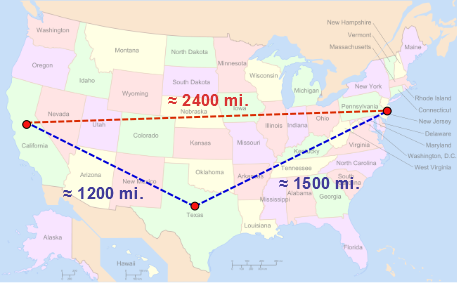
One can imagine the triangle inequality as saying the following: you will go fewer miles flying a plane from New Jersey straight to California than you would if you flew from New Jersey to Texas and then to California.
Let's summarize these things formally:
Definition (Metric). A metric on a space $X$ is a function $d:X\times X\to {\mathbb R}_{\geq 0}$ which takes as input two points in $X$ and gives a non-negative real number, and for which the following holds:
- For $x,y\in X$, $d(x,y) \geq 0$, and $d(x,y) = 0$ if and only if $x = y$.
- For $x,y\in X$, $d(x,y) = d(y,x)$.
- For $x,y,z\in X$, $d(x,z)\leq d(x,y) + d(y,z)$.
Not every topological space can have a metric on it, but we won't talk about this now. If a space happens to have a metric associated to it, we call the space (and its associated metric) it a metric space. Most of the spaces that occur in the "real world" are metric spaces; any ${\mathbb R}^{n}$ is a metric space with the distance function as a metric. For the most part, we will only use this latter space &mdash we even give the distance function a neat new name when it's on ${\mathbb R}^{n}$: the standard Euclidean metric. Formally,
Definition (Standard Euclidean Metric). Let $x = (x_{1}, x_{2}, \dots, x_{n})$ and $y = (y_{1},y_{2},\dots, y_{n})$, both in ${\mathbb R}^{n}$. The Standard Euclidean metric on ${\mathbb R}^{n}$ is defined as \[d(x,y) = \sqrt{\sum_{i=1}^{n}(x_{i}-y_{i})^{2}}.\]
That is, you take each component, square the difference, add all that up, and take the square root. For $n = 1,2,3$ you should see that this, indeed, gives you the standard distance function you're used to.
[Note that $|x| = \sqrt{x^{2}}$ for the case $n=1$.]
Čech Complexes in ${\mathbb R}^{n}$.
At this point, we ought to talk about open balls about a point, which are often the open sets of choice when working in ${\mathbb R}^{n}$ with the standard Euclidean metric. We define an open ball about a point as follows:
Definition (Open Ball). Given a point $x\in {\mathbb R}^{n}$ and a real number $r>0$, we call all points a distance less than $r$ away from $x$ the ball of radius $r$ about $x$ and we denote it $B_{r}(x)$. That is, \[B_{r}(x) = \{y\in {\mathbb R}^{n}\,|\,d(x,y)\lt r\}.\]
For example, in ${\mathbb R}^{1}$ they form open intervals like $(x-r, x+r)$. In ${\mathbb R}^{2}$ they are solid circles without the outside circle boundary centered at $x$ with radius $r$. In ${\mathbb R}^{3}$ they are solid spheres without the outer boundary centered at $x$ with radius $r$. In all of these cases, they form particularly nice, particularly symmetric open sets which we can use to easily cover spaces.
In general, we're guaranteed at least one (not necessarily good) cover: given some space $X$, take the collection of open balls of radius $r>0$ about every single point in $X$. This cover is somewhat special, so we will denote it by \[{\mathcal B}_{r}(X) = \{B_{r}(x)\}_{x\in X}.\]
The following theorem will mean something to you if you know what a compact Riemannian manifold is and what homotopy equivalence means; if not, just skip over it.
Theorem. Let $M$ be a compact Riemannian manifold. There here exists some $e>0$ such that ${\mathcal B}_{r}(M)$ is a good cover of $M$ whenever $r \leq e$ so that $N({\mathcal B}_{r}(M))$ is a Čech Complex; in addition, we have that $N({\mathcal B}_{r}(M))$ is homotopy equivalent to $M$ in this case. Moreover, for each $r\leq e$, there is some finite set of points $V$ so that the subcomplex $N({\mathcal B}_{r}(V))$ is homotopy equivalent to $M$.
Said another way: if our space is nice enough then there exists a good cover which is given by ${\mathcal B}_{r}(X)$ for some $r$ and, even better, there is some finite set of points $V$ such that ${\mathcal B}_{r}(V)$ (which will be a finite cover!) whose associated Čech Complex will retain the general topological structure of the original space.
The Vietoris-Rips Complex.
This is great and all but there's a few problems with the Čech Complex. First, the idea is fantastic theoretically, but practically, even if we are working with a simple 2-dimensional circle or a line segment, ${\mathcal B}_{r}(X)$ will be an infinite set as we are working with an infinite number of points. Clearly, we will want to only work with finitely many of those points — but which should we choose? It's not always clear. In addition, the construction is quite computationally expensive and, sometimes, needlessly so: for example, consider the picture below:

Pretend this is one small piece of some larger structure but that in this small area the space is smooth, nice, and there's no holes in it anywhere. The blue disks are part of the open cover of the space in this area. Notice how many times they intersect! In particular, each of these intersects with all of the others which means there will be: seven $0$-simplices, twenty-one $1$-simplices, thirty-five $2$-simplices, thirty-five $3$-simplices, twenty-one $4$-simplices, seven $5$-simplices, and one $6$-simplex. On the other hand, taking a single open set (with the exact same coverage as our previous open sets!) like this:

gives us a single $0$-simplex. There seems to be some unnecessary redundancy when it comes to covering things arbitrarily. To attempt to remedy this problem we will introduce a new complex called the Vietoris-Rips Complex, which we will compare with the Čech Complex. Luckily, we've already learned most of what we need to define the Vietoris-Rips complex.
Let's work in ${\mathbb R}^{n}$ with the standard Euclidean distance. We're going to use the following "reasonable" idea: two vertices should be joined by an edge if they're close to each other. Specifically, given some small positive number, which we'll call $\epsilon$, if $d(v_{1},v_{2}) \leq \epsilon$ then we'll put a $1$-simplex (an edge) between $v_{1}$ and $v_{2}$. Similarly, if three vertices are all close to each other, we'll make them the vertices of a $2$-simplex; that is, if $d(v_{1},v_{2}), d(v_{1},v_{3}),$ and $d(v_{2},v_{3})$ are all $\leq \epsilon$ then we'll make $v_{1},v_{2},$ and $v_{3}$ the vertices of a $2$-simplex.
It's straightforward how to continue, so we'll formalize this now and then we'll do a bunch of examples.
Definition (Vietoris-Rips Complex). Let $X$ be a subset of a metric space [we will focus on subsets of ${\mathbb R}^{n}$ in this post] and let $d$ be its metric. Pick an $\epsilon > 0$. Construct a simplicial complex as follows:
- Add a $0$-simplex for each point in $X$.
- For $x_{1},x_{2}\in X$, add a $1$-simplex between $x_{1},x_{2}$ if $d(x_{1},x_{2}) \leq \epsilon$.
- For $x_{1},x_{2}, x_{3}\in X$, add a $2$-simplex with vertices $x_{1},x_{2}, x_{3}$ if $d(x_{1},x_{2}), d(x_{1},x_{3}),d(x_{2},x_{3}) \leq \epsilon$.
- $\dots$
- For $x_{1},x_{2},\dots, x_{n}\in X$, add an $n$-simplex with vertices $x_{1},x_{2},\dots x_{n}$ if $d(x_{i},x_{j}) \leq \epsilon$ for $0\leq i,j\leq n$; that is, if all the points are within a distance of $\epsilon$ from each other.
This simplicial complex is called the Vietoris-Rips Complex and is denoted $VR(X,\epsilon)$.
Let's do some examples and then we'll talk about how it compares to the Čech Complex.
Examples of Vietoris-Rips Complexes.
The Vietoris-Rips Complex depends in a cruicial way on the choice of the radius of the balls we use. For example, the following space uses a small radius:

As a Čech Complex this would have four $0$ simplices and four $1$-simplices (make this!), but as a Vietoris-Rips complex no point is close enough to any other to make any $1$-simplices. Hence, the Vietoris-Rips complex is just four $0$-simplices. Sad. Let's make the radius a bit bigger and see what happens.

This looks more interesting. The Vietoris-Rips complex is shown here as four $0$-simplices and four $1$-simplices. The corresponding Čech Complex, in addition to these simplices, would also have four $2$-simplex and a single $3$-simplex. If we make the radius still bigger, we will obtain:

This will have the same Čech Complex as before, but now there is enough overlap to have a few $2$-simplices bounding a $3$-simplex (this is, therefore, a solid tetrahedron). In fact, here, our Čech Complex and our Vietoris-Rips complex are the same structure. Pretty neat.
Let's do another example, just for a bit more practice. Let's make it a bit more interesting by adding another point; nothing too crazy yet! Let's start with small radius balls:

Our Vietoris-Rips complex will just be these five $0$-simplices. Kind of dull. [For practice, you may want to make the Čech Complex.] Now let's make the radius a bit larger:

This gives us a slightly neater looking Vietoris-Rips complex: we now have a $3$-simplex and all of the required $2$- and $1$- simplices to bound the $3$-simplex:

But there is still a lonely point all the way on the right. It looks pretty lonely, so let's increase the radius a bit to include it:

Neat. If we were to make the radius a bunch larger, what would happen? We would eventually get a large $4$-simplex (why?) containing each of the points as vertices.
[Note: if you're feeling particularly masochistic, you should feel free to compute the associated Čech Complexes for the above covers. You may want to make them abstract simplicial complexes, since larger dimensional simplices are difficult to draw.]
Notice something here: the size of the radius affects the Vietoris-Rips complex. Different sizes for the radius will tell us different tihngs about the points: in particular, in this above example, it tells us that these four left-hand points are much closer to each other than they are to the point on the right. Both of these examples were quite similar, so let's have one which shows us something a bit more interesting:

These points are arranged in a circular form; we'd like, at some point, our Vietoris-Rips complex to tell us this. Let's start with a small radius, but not so small that each open set only covers one point each (since that's a bit boring),

You may want to try to make this yourself on a piece of paper. We note that we will have a total of eight $0$-simplices, sixteen $1$-simplices, eight $2$-simplices [I've drawn these as yellow and green just to distinguish them, but they're all just regular $2$-simplices], and no $3$-simplices. It's a bit tricky to see, but the Vietoris-Rips complex at this point almost looks like a ring that one could wear on one's finger.
If we make the radius larger, we will eventually start making $4$-simplices (and the $3$-, $2$-, and $1$-simplices which bound it) in the same sort of ring-type way — though, this is impossible to draw, so I'll leave it to your imaginations. If we make the radius a bit bigger, we get a ring of $6$-simplices (and the simplices which bo und it), and, last, when we make the radius quite large so as to contain each point in every open ball we will obtain an $8$-simplex (with all the simplices which bound it). There are, of course, not easy to imagine, but, mathematically, they will tell us something. For example, with the exception of the largest radius we tried and the smallest radius (which each just contained one $0$-simplex each) each of these has the homotopy type of a circle; that is, topologically, they have many of the same characteristics that a circle has.
We will formalize the idea of homotopy type in a section below, but for now we should note something: the points, even though they were not connected to each other at first, "looked" like a circle to us. The ability to think that something "looks" like something else is quite difficult to program a computer to be able to do. When we made our Vietoris-Rips complex, we did nothing but increase the radius of the open balls covering them and eventually found a structure which was, topologically, quite similar to a circle. Because computers can compute distances and compute homotopy types of simplicial complexes, building this kind of structure is something that a computer can do.
This is the crucial point to keep in mind: using these structures, we can use computers to find out what data "looks like."
What about the Čech Complex?
Interestingly, we have a nice relationship between the Čech Complex and the Vietoris-Rips Complex. We'll have to work in Euclidean space, ${\mathbb R}^{n}$, with the standard metric and we'll only be able to use standard open balls as our open sets (since this is how we defined the Vietoris-Rips complex). The idea is that the Vietoris-Rips complex is somehow "inbetween" two Čech Complexes for $X$. Specifically:
Given some $\epsilon>0$, if the cover ${\mathcal B}_{\epsilon}(X)$ happens to be a good cover then the associated Čech Complex ${\mathcal N}({\mathcal B}_{\epsilon}(X))$ is defined. Moreover, if the cover ${\mathcal B}_{2\epsilon}(X)$ happens to be a good cover, then ${\mathcal N}({\mathcal B}_{\epsilon}(X))$ is also defined. We always have that the Vietoris-Rips complex $VR(X,2\epsilon)$ is defined (but isn't always pretty to look at!), and the magic is the following:
Proposition. Let $X$ be a metric space. If, for some $\epsilon > 0$ we have that ${\mathcal B}_{\epsilon}(X)$ and ${\mathcal B}_{2\epsilon}(X)$ are both good covers, then we have the following inclusions: \[{\mathcal N}({\mathcal B}_{\epsilon}(X))\subseteq VR(X,2\epsilon) \subseteq {\mathcal N}({\mathcal B}_{2\epsilon}(X)).\]
As usual, we won't prove this but we will show an example of this happening. Let's do a simple one and a more complicated one. First, let's look at a triangle of points with a relatively small radius $\epsilon > 0$. Notice that this is a good cover. Second, notice that the Vietoris-Rips complex of this is simply the three points. Kind of boring.

Let's construct the Čech Complexes for this cover! Here is ${\mathcal N}({\mathcal B}_{\epsilon}(X))$:
A bit boring; it's just the $0$-simplices. Let's find the Vietoris-Rips complex for $2\epsilon$. We should have that the first Čech Complex is a subcomplex of it.

Note that this also happens to be the Čech Complex for $2\epsilon$. Hence, our inclusions work: the $0$-simplices certainly are a subcomplex of the Vietoris-Rips complex for $2\epsilon$, and the Vietoris-Rips complex for $2\epsilon$ and the Čech Complex for $2\epsilon$ are identical, so the first is trivially a subcomplex of the latter.
But maybe you didn't think that structure was interesting enough to show off any differences. You're not alone! It's a pretty dull structure. Let's do a slightly different one, drawn below with, as usual, the $\epsilon$-balls already drawn in.

First, note that this cover is a good cover. Next, let's build up the Čech Complex (try this before you look below!):

Slightly neater. At least there's a nice $2$-simplex in there. Now, let's draw the $2\epsilon$ open sets:

Note that this is a good cover. The interested reader, at this point, should construct for themselves the associated Čech and Vietoris-Rips Complexes. I'll do the Vietoris-Rips complex first:

Note that this is the same as our $\epsilon$ Čech complex, so the first inclusion holds! Neat. Now the (much more complicated) Čech Complex for $2\epsilon$.

Notice that there is a $3$-simplex on the left-hand side where there was only a $2$-simplex in the Vietoris-Rips complex for $2\epsilon$; nonetheless, the Vietoris-Rips complex is still a subcomplex of this complex. The inclusion holds for this slightly more interesting structure. We'd expect this, since someone did a lot of hard work to prove that proposition above!
What does this proposition mean? It means that we can use the Vietoris-Rips complex and still get the information that the Čech Complex would have given us, so long as we vary our use of $\epsilon$'s (taking a range of small, medium, and large-sized $\epsilon$'s for example). Notice that, in relation to the Vietoris-Rips complex, the Čech complex almost always has extra simplices hanging out all over the place which (in practice) don't add much to our analysis of the space. Hence, we ought to give up on using the Čech complex for a while and focus our efforts on the Vietoris-Rips complex. Until something better comes along, at least.
So, are there any problems with the Vietoris-Rips Complex?
Yes. First of all, note that in all of the calculations we've done we've used a small number of points. On the other hand, if you're trying to make a Vietoris-Rips complex for, say, a circle (which has infinitely many points) you'd need infinitely many $0$-simplices. More realistically, if you had a large number of data points, we'd need to store a large number of $0$-simplices; this is computationally expensive, especially if you only want the gist of the data. As a telling example, consider the following example:

We'll draw an example of what the Vietoris-Rips complex might look like in this case with a relatively small radius $\epsilon$ (the brave reader might want to think about what the associated Čech complex might look like!),

[I may have missed a few $1$- or $2$-simplices here; blame it on doing this by eye instead of computing it!] It may be the case that this analysis is a particularly nice one and the Vietoris-Rips complex has told us something — on the other hand, these may be two small clusters in a much larger collection of data: perhaps all we want to say, in this case, is that this piece of the data forms two nice little clusters. In that case, we don't need so many $0$-cells, $1$-cells, $2$-cells, etc; we could represent these two clusters by, perhaps, two $0$-cells. Wanting to "fix" this problem in the Vietoris-Rips complex leads us to a new idea: perhaps $\epsilon$-balls aren't the best way to talk about neighboring points. They're a bit too restrictive sometimes when it comes to clusterings. What we'd like is something like the following: make a few points (in red, in my drawing) and associate with this point the $0$-simplices most near to it.

The reader may wish to pause for a moment and try to think of a way to proceed. There are many different ways; we will pick the one which the author feels is most elegant.
Voronoi Again (Naturally).
Sets of points nearest to some point is a common problem, which is lucky since there are already structures which solve this problem. We've even talked about it before; the structures we will be using are called Voronoi Diagrams and Delaunay Triangulations. We will not be completely be throwing out the Vietoris-Rips diagrams (lest the reader think we start building up concepts just to trash them when something new and exciting comes along!) but these will give us ways to make our data more refined so that the Vietoris-Rips diagrams will be computationally easier to handle.
If you remember what Voronoi diagrams are, feel free to skim this part until the horizontal line below. The general idea about Voronoi diagrams is: given a set of points, we cut up the plane into little "fenced in" areas such that each point is in the fenced in area with points that are closer to it than any other point. A picture might explain this a bit better:

In the picture above, the red area is made up of points which are closer to point 1 than they are to points 2 or 3. Similarly, the blue area is made up of points closer to point 2 than points 1 or 3. We call the green, red, and blue areas Voronoi polygons; they each will contain exactly one point from the set we look at (by definition).
How does this help us with Vietoris-Rips diagrams, though? Note that all of the Voronoi polygons form an open cover of the points.
[For those who care: actually, it almost forms an open cover; there are little pieces (along the boundaries) which this cover doesn't cover. Luckily, it doesn't affect much to "stretch" this cover over the boundary; that is, formally, we could "thicken" the boundary to some open $\epsilon$-tube and union pieces of it with each of the Voronoi polygons. For a planar diagram, and for finite points, it is always possible to do this; we just leave the messy details for those who need to write papers on this.]
In the other post, we obtained the Delaunay triangulation corresponding to the Voronoi diagram by taking the dual of the Voronoi diagram; this time, we can talk about it in a slightly different way. Recall the notion of a nerve from the previous post (this is how we defined Čech Complexes corresponding to a (good) open cover). For each open set, we place an associated $0$-simplex; for each non-empty intersection of two open sets, we place a $1$-simplex; for each non-empty intersection of three open sets, we place a $2$-simplex; and so on and so on. The attachments are the obvious ones: a $1$-simplex will be attached to the two $0$-simplexes corresponding to the open sets which were intersected to get the $1$-simplex. Let's try to do this to our Voronoi diagram above, recalling that we will consider the intersection of the two neighboring open Voronoi polygons to be their common boundary (which is almost true; see note above).

We notice that this makes a (squished around) $2$-simplex, with all of its edges and vertices. Neat.
Now, let's get to the point of using these structures. Because it will be instructive to do an example first, let's do exactly that. Remember our old friend, "two clusters of points"? Well, let's pretend that there's a few more clusters...

Notice that our feeling here is that these clusters are sort of in a circular kind of arrangement. Notice, also, that most standard methods of data analysis which are computation would probably miss this: it's not linear, it's not quadratic; it's not polynomials, in general. If we place what we'll call a landmark point at each of the clusters (think of these as being the ladymarks which tell us which cluster we're in if we were driving around on the plane), then our diagram becomes much simpler:

Let's make this a Voronoi diagram! It's going to look something like this:

And from this, we can take the nerve of the cover of Voronoi polygons and get the corresponding Delaunay triangulation.

Though this looks a bit strange, it does have the homotopy type (it, topologically, looks like) a circle. This tells us that our data, topologically, "seems" like a circle. This was a rough sketch, as well: the landmark points were arbitrarily chosen to be "near" all the data it represents; there is, perhaps, a more rigorous way to do this. Nonetheless, the idea is clear: clusters can be represented by landmark points, which reduce computations and allow us to create a simplex which represents the topological structure of the data.
The reader may be exhausted by this point. So many complexes! So many nerves! We'll stop here and let the reader take a breath.
Next time...
Next time, we need to talk about orientation of simplicial complexes. After this, we'll discuss the foundations to computing homology: boundaries and cycles. From there, we'll be at a point where we can compute the homology of our structures and be able to tell what they "look like" topologically!