DyingLoveGrape.
The F-distribution.
Prereqs.
You should be pretty familiar with some basic statistics for this post. In particular, you should have seen hypothesis testing (difference of single means, at least), and you should know what a null hypothesis is. The largest piece, which is optional but important, is knowing about Chi Squared distributions; you should read about these a bit if you'd like to know exactly what's going on. I'll try not to assume too much more knowledge.
also, with each plot that I have in this post, clicking it will link you to the (usually R) source code so you can try things yourself!
Introduction.
Sometimes people will talk about the F-distribution or the F-test; this is a bit misleading. It gives the reader the idea that there is only one F-test or F-distribution — but this is not the case. The term F-test applies to any test where the associated test statistic has an F-distribution under the null hypothesis; that is, any test where assuming the null hypothesis will make it so that the thing we're testing has the F-distribution. An F-distribution is dependent on two values (called the degrees of freedom) which will change its shape. It wouldn't be easy to talk about an F-test without discussing the F-distribution, which is why the next section is called —
The F-distribution.
First, a bit of motivation. How do we tell if two values (say, real numbers) are the same? We usually will say $x = y$, but, if $x, y$ are not zero we can also say $\frac{x}{y} = 1$. This has the added bonus of being able to be applied to functions: $\frac{f(x)}{g(x)} = 1$. In this way, instead of saying $f(x) = g(y)$ when $x = y$, we can construct a new function $h(x) = \frac{f(x)}{g(x)}$ and see whether $h(x) = 1$ (usually almost everywhere).
In "real math", a random variable is a function which takes on a value with some probability. We call any particular outcome the random variate. So, for example, if we have $U_{1}$ is a Chi-squared variate with degrees of freedom $d_{1}$, this means that it is some particular value that comes out with a probability defined by the Chi-squared distribution with degrees of freedom $d_{1}$. (We'll do an example of this in a minute if you aren't quite catching onto all this lingo.)
Now, what if we have two Chi-Squared distributions, $U_{1}, U_{2}$, with degrees of freedom $d_{1}, d_{2}$ respectively. Are they going to be equal most of the time? Odds are, probably not. But that's okay. We can see how close they are to each other by dividing them (remember? from before?). We'll include the degrees of freedom as well (mainly for reasons of normalization; you don't need to worry much about why we do this), and create a new random variable: \[X = \dfrac{\dfrac{U_{1}}{d_{1}}}{\dfrac{U_{2}}{d_{2}}}\] and the associated variate will just be to get variates from $U_{1}, U_{2}$ and divide them. This new random variable $X$ is, in other words, created by taking the ratio of two Chi-squared random variables. Neato.
[As a note here, we also require that these Chi-square variables to be independent, as with most statistical tests.]
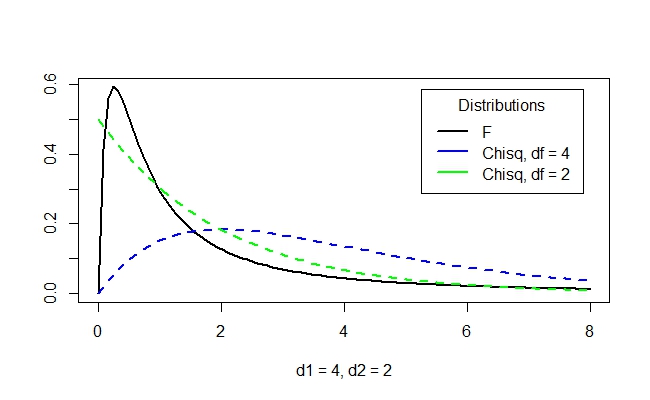
I've plotted two different Chi-squared distributions below, and their associated F-distribution (what we've called $X$ above):
and here's a slightly different F-distribution with two different degrees of freedom:
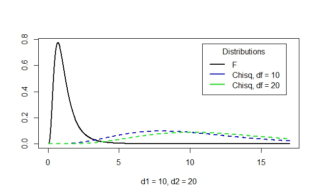
This should show you that making the F-distribution is not just as easy as multiplying (pointwise) the two chi-square distributions! The general shapes of the F-distributions look like this:
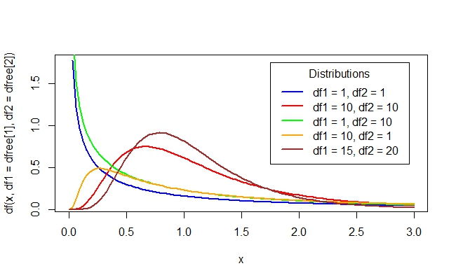
We see some standard patterns coming out of these distributions: we either get this graph with a asympote near the origin or we get this graph with a little hump near the origin.
Now that we know what these look like, let's ask the following question: supposing that one distibution we have is Chi-Squared $U_{1}$ with $df = 4$ and another which is Chi-Squared $U_{2}$ with $df = 2$ (as in the first figure above). What are the chances that for \[X = \dfrac{\dfrac{U_{1}}{4}}{\dfrac{U_{2}}{2}}\] we have $2 \leq X \leq 4$? Unpacking this, we see the following idea: we'd have to have \[U_{2} \leq \frac{U_{1}}{4} \leq 2U_{2}\] (Why? We look at the inequality, replace $X$ with its actual expression, then multiply both sides by $\frac{U_{2}}{2}$.) This is, of course, \[4U_{2} \leq U_{1} \leq 8U_{2}\] so the question becomes: given some value of $U_{2}$, how often is $U_{1}$ between $4U_{2}$ and $8U_{2}$. This question is a bit more complicated, though: the "given some value" is a bit misleading; we are given values according to the probabilities inherent in $U_{2}$. Lots and lots of mathematics goes into this, but the punch line is that we can figure this out by looking at the associated $F$-distribution. We ask: how often is the $F$-distribution between 2 and 4? We use a computer to figure this out for us (more on this later):
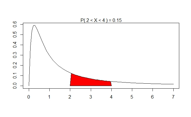
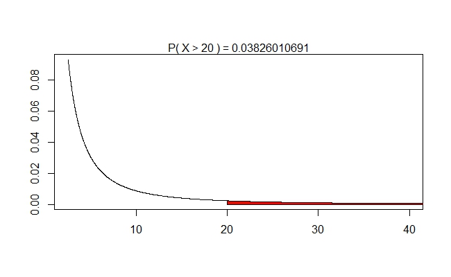
Notice that this happens about $15\%$ of the time (given at the top of the graph). We'd perhaps expect thins kind of thing, given the graphs of the Chi-Squared distributions. Let's ask now, jut for kicks, how probable is it to have $X > 20$? We'd have to have \[U_{1} \geq 40U_{2}\] and, since most of the time our $U_{2}$ will be hovering between 5 and 17, we'd need our $U_{1}$ to hover between 200 and 680. Judging from the graph of $U_{1}$, this will not happen often. Hence, we intuitively think this should happen very rarely. The computer will confirm these suspicions:
One thing that makes the probably so much higher than you might imgine is that $U_{2}$ will also spend some time being quite tiny (less than 1) and so it will give a chance for $U_{1}$ to be in a reasonable range. Most of the area, of course, is located between 0 and 4. This interval is responsible for about $80\%$ of the area.
The F-Test in One-way ANOVA, or: "why should I care about the F-Distribution?"
You may have said to yourself in the last section, "So what?" a couple of dozen times. The F-distribution is nice, sure, but what can we use it for? When am I going to find myself in a position where I need to look at the ratio of two Chi-Squared random variables divided by their respective degrees of freedom?
Here's where you need to know something about chi-square distributions. In particular, we can define the chi-square distribution as follows: given $Z_{i}$ is a standard normal distribution (one where $\mu = 0$ and $\sigma = 1$) we have that \[X = \sum_{i=1}^{k}Z_{i}^{2}\] has a chi-square distribution with $k$ degrees of freedom. This means that if we have a whole bunch of variates from standard normal distributions, square them, then add them up, we'll get a chi-squared variate (by definition). So, here's where we introduce two new concepts.
Suppose we are given a few groups of data, $A_{1}, A_{2}, \dots, A_{m}$, each with $n$ data points each sampled from a normal distribution. Suppose that group $A_{i}$ has mean $\mu_{i}$ and that, if we added all the data from all the groups together and took the mean, we'd get $\mu$. Then...
The between-group Sum of Squares is calculated by replacing each point in $A_{i}$ with $\mu_{i}$, then taking the difference between $\mu_{i}$ and $\mu$ and squaring it. In other words, \[\begin{align*}S_{between} &= (\mu_{1} - \mu)^{2} + (\mu_{1} - \mu)^{2} + \dots + (\mu_{1} - \mu)^{2} + (\mu_{2} - \mu)^{2} + \dots + (\mu_{m} - \mu)^{2}\\ &= n(\mu_{1} - \mu)^{2} + n(\mu_{2} - \mu) + \dots + n(\mu_{m} - \mu)\\ &= n[(\mu_{1} - \mu)^{2} + (\mu_{2} - \mu)^{2} + \dots + (\mu_{m} - \mu)^{2})]\\ \end{align*}\] In essence, this measures the distance of the average of each group from the average of all of the data points. For instance, if all of the groups have similar values, the $\mu$ will be close to the common average and $S_{between}$ will be fairly small. Conversely, if the groups have crazy different averages, there will be a larger amount of variation of each from $\mu$ giving us a larger $S_{between}$.
The within-group Sum of Squares is similar, but it looks at how far the points in each group vary from their respective means. The way to make notation for this this is a nightmare, but it will go something like this. Suppose that $A_{1} = \{a_{1}, a_{2}, \dots, a_{m}\}$ and $A_{2} = \{b_{1}, b_{2}, \dots, b_{m}\}$ and, as before, the mean of $A_{1}$ is $\mu_{1}$ and the mean of $A_{2}$ is $\mu_{2}$. We then find \[(a_{i} - \mu_{1})^{2}\] for each value $a_{i}$ in $A_{1}$ and add them together. Then we do the same thing for $A_{2}$; we find \[(b_{i} - \mu_{2})^{2}\] for each value $b_{i}$ in $A_{2}$ and add them together. Then, we add this value to the value we got for $A_{1}$. If we had another set, we'd do the same thing, and add this value on as well. (If you're a bit more experienced in stats, you may want to rewrite this definition in terms of $\sigma^{2}_{i}$, the variance of $A_{i}$.) We'll do an example of this soon, so don't worry if you're not entirely confident with this one yet. We denote this value by $S_{within}$.
The idea behind this revolves around the idea of variance: if the elements in each group are close to their group's mean, then they will contribute little to $S_{within}$. If, on the other hand, the elements are wildly spread out in each group, they will cause $S_{within}$ to be larger.
Last (I know, I said only two definitions, but these last ones are easy!), we define the mean between-group Sum of Squares, which is $MS_{between} = \dfrac{S_{between}}{m-1}$ where $m$ is the total number of groups, and the mean within-group Sum of Squares, which is $MS_{within}=\dfrac{S_{within}}{m(n-1)}$ where $m$ is the total number of groups and $n$ is the number of elements in each group. The reason for the strange $-1$ here is due to some degrees-of-freedom stuff that makes the calculations work out — don't worry much about it.
So what about F? We take these two values and create: \[F = \frac{MS_{between}}{MS_{within}}\] which we call the F statistics. Yes, that F statistic! Look back and see that this definition jives with what we defined an F statistic to be before.
Important Point: if all of the $A_{i}$ groups were representative samples picked from the same populations, we'd expect that the variance in each $A_{i}$ to be pretty close to the variance of all of the elements together (which would, in turn, approximate the variance of the population). Hence, looking at the ratio of $MS_{between}$ and $MS_{within}$ is a good way to measure how well or poorly the data looks like it is a (somewhat) representative sample from the same population. Purists will note that this is not "exactly" true, but it is good to motivate why we'd want to look at these values and form these fractions.
Also notice that if we assume $A_{i}$ to be from a standard normal distribution then all of these differences that we've been taking are variates from chi-squared distributions! In sum, this means we can use the F value to talk about this nonsense. Let's think about this by doing an example.
A Delightful ANOVA Example.
Let's say we have the following two samples of data that we want to test to see if they came from the same distribution (you can think of this as a "before-and-after" test, and we'd like to say that there is no change between 'before' and 'after'): \[\begin{array}{|c|c|}\hline A_{1} & A_{2}\\ \hline 4 & 6\\ 2 & 7\\ 2 & 10\\ 2 & 1\\ \hline \end{array}\] In this case they don't look all that similar but let's test them formally. Let's just calculate a few things here before we begin. We have: \[\begin{align*} \mu_{1} &= 2.5,\\ \mu_{2} &= 6,\\ \mu & = 4.25\\ \end{align*}\] We notice that the first group of numbers is fairly close to $\mu_{1}$ so it won't make much of a contribution to $S_{within}$, but the second group is all sorts of spread out. We'll see that it will be the primary contributer to $S_{within}$. Neither $\mu_{1}$ nor $\mu_{2}$ is particularly far from $\mu$, but we'll see how close they "ought" to be.
Let's compute some things here. We have that, \[\begin{align*} S_{between} &= 4[(2.5 - 4.25)^{2} + (6-4.25)^{2}]\\ &=4[3.0625 + 3.0625] = 24.5 \end{align*}\] and, therefore, \[MS_{between} = \frac{24.5}{1} = 24.5.\] Similarly, but more irritatingly, we figure out $S_{within}$. We need to make a new table since we're subtracting from each element: \[\begin{array}{|c|c|}\hline A_{1} & A_{2}\\ \hline 4-2.5 & 6-6\\ 2-2.5 & 7-6\\ 2-2.5 & 10-6\\ 2-2.5 & 1-6\\ \hline \end{array}\] which, reducing, gives us: \[\begin{array}{|c|c|}\hline A_{1} & A_{2}\\ \hline 1.5 & 0\\ -0.5 & 1\\ -0.5 & 6\\ -0.5 & -5\\ \hline \end{array}\] and squaring each entry gives us: \[\begin{array}{|c|c|}\hline A_{1} & A_{2}\\ \hline 2.25 & 0\\ 0.25 & 1\\ 0.25 & 36\\ 0.25 & 25\\ \hline \end{array}\] Note that, as we said before, the contribution of $A_{1}$ is pretty small (only 3), but the contribution of $A_{2}$ is gigantic! We have that: \[\begin{align*}S_{within} &= 2.25 + 0.25 + 0.25 + 0.25 + 0 + 1 + 36 + 25\\ &=65 \end{align*}\] and, consequently, \[MS_{within} = \frac{65}{2(4-1)} = \frac{65}{6} = 10.83\] which gives us the ratio \[F = \frac{MS_{between}}{MS_{within}} = \frac{24.5}{10.83} = 2.26.\]
Now what? As usual, we will look at the associated F-distribution. Here, on top we have the "between" degrees of freedom which was $df_{1} = (m-1) = 1$, and on the bottom we have the "within" degrees of freedom which was $df_{2} = m(n-1) = 2(3) = 6.$ We now form the F-distirbution with these degrees of freedom:
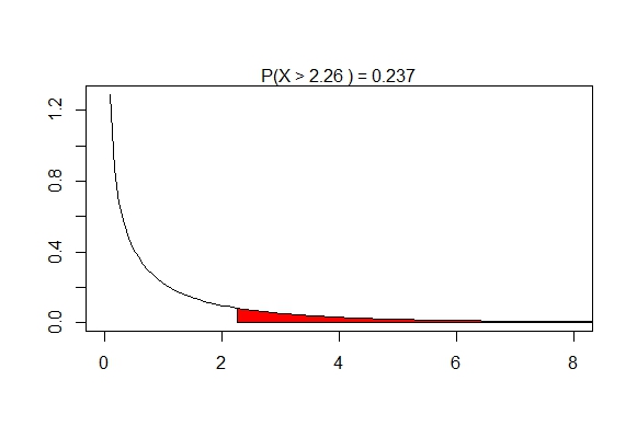
We obtain a $p$-value of 0.237, which is not enough to say these values aren't from the same population. Alas. Interestingly, the data do look different in each group, but it may be the case that there simply weren't enough data points to rule out the case that they were samples from the same distribution. Note that to find the $p$-value, you would normally use a computater, a calculator, or a chart; this isn't something you can easily calcuate with pen-and-paper on your own.
One More Example.
Let's do an example that's a bit more extreme. Let's suppose we have \[\begin{array}{|c|c|}\hline A_{1} & A_{2}\\ \hline 2 & 10\\ 2 & 10\\ 2 & 10\\ 2 & 10\\ 2 & 10\\ 2 & 10\\ 2 & 10\\ 2 & 10\\ 2 & 10\\ 0 & 0\\ \hline \end{array}\] Notice the last two values in each group are both 0. It seems like these two groups probably won't be from the same population, but let's do some calculations. We have $\mu_{1} = 1.8$, $\mu_{2} = 9$, and $\mu = 5.4$. Our $S_{between}$ is fairly easy to compute: \[\begin{align*}S_{between} &= 10[(1.8 - 5.4)^{2} + (9 - 5.4)^{2}] \\ &= 10[12.96 + 12.96]\\ &= 259.2\end{align*}\] But our $S_{within}$ is a bit more irritating to compute. You can compute it the long way, but I'll just note that $S_{within} = 3.6 + 90 = 93.6.$
This means that we have \[MS_{between} = \frac{259.2}{1} = 259.2\] \[MS_{within} = \frac{93.6}{2(9)} = 5.2\] which means that \[F = \frac{MS_{between}}{MS_{within}} = \frac{259.2}{5.2} = 49.85.\]
If we plot this (using the degrees of freedom 1 and 9 respectively),
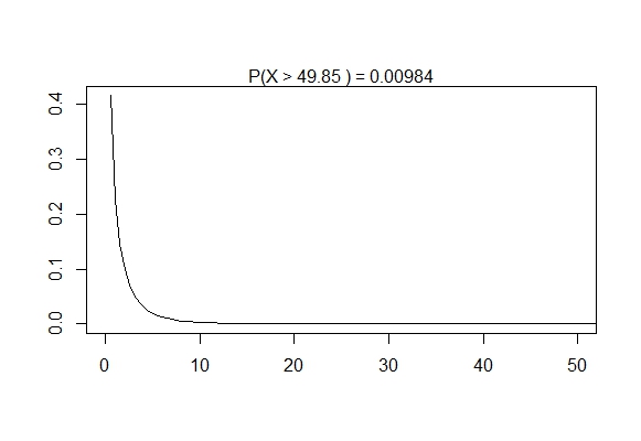
Note that the $p$-value is 0.0098. This is way below 0.05, our usual signifance level, so we can say that we are fairly confident that these two samples did not come from the same distribution. This seems pretty reasonable looking at the data, even noting that there are only ten data points in each group.
A bit more formally,...
We can formalize most of this. We can say that, given the same equations as above, $F = \frac{MS_{between}}{MS_{within}}$ and that the associated $p$-value will be $P(X > F)$ where $X$ is a random variable with the F-distribution with the associated degrees of freedom. Sometimes you'll see this as $F_{df1, df2}$ with the degrees of freedom attached. As usual, the $p$-value is useful when testing at some significance level $\alpha$; in this case, we have:
\[H_{0}: \mbox{The groups represent the same (normal) distribution.}\] \[H_{A}: \mbox{At least one group does not represent the same (normal) distribution.}\]Here, we needed to note that these groups were assumed to be normal. This is needed for the null hypothesis since the chi-squared distributions (which make up the F-distribution) are, by definition, sums of squares of normal distributions.
Sometimes these conclusions are put differently. If we know that the variance of the three groups are the same or close enough (or if we assume this) then we can use this test to see if the means are all approximately the same (or, if they are reasonably close). Similarly, if we know the means of the three groups are close enough then we can see if the variances of the groups are close. This latter case is the idea behind most of the analysis we've done so far.
What else?
We've touched upon the most basic F-test: the one for one-way ANOVA tests. We can squeeze a bit more use out of the F-distribution, but only if begin to look at ANOVA. Indeed, ANOVA and its closely-related friends are probably some of the most popular and important tools in analyzing data for nearly every data-heavy field. We'll soon see why.